1 2 3 4 5 6 7 8 9

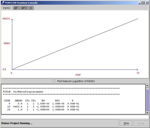
48) After Competing the project Run the Project by selecting "Run Project" Option from Run Menu at the top. It will start a Runtime console window as shown in fig 5.9.

Fig - 5.9: Runtime Console for the Project.

Here during run time graphs for change in value of different variables can be seen by selecting the tabs( at top). The project can take time to complete depending upon the problem. After Completion the following message box will appear asking for loading the solution file for postprocessing as shown in fig 6.0.

Fig - 6.0: Load Solution file Message Box

49) Click Yes to load the Solution file and Post Process the project.

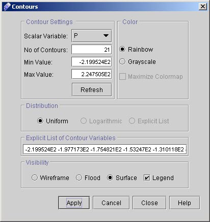
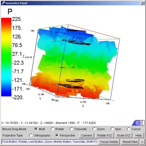
50)Click "Contours" and uncheck Grid. A dialog window will appear. (See fig 5.0). From this window you can choose different option for contour plot of dependent variables. Choose scalar variable "P" and click on flood. The resulting plot with Legend option is shown in Fig.6.1.

Fig - 6.1: Contour Options For P

Click Apply when finished.

51) The resulting plot with Legend option is shown in Fig.6.2.

Fig - 6.2: Surface Plot For P

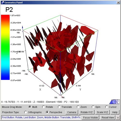
52) Similarly get Plot for P2. The Plot for P2 by selecting the scalar variable P2. Plot should look like as shown in fig 6.3.

Fig - 6.3: Surface Plot For P2

This concludes this PORFLOW™ tutorial. There are other pre and Postprocessing features that are not covered herein, so please make sure to check all screens and tabs to see it for yourself.

1 2 3 4 5 6 7 8 9

# Back to CFDStudio/PORFLOW Tutorials Page

Related Links:

# PORFLOW Applications
# PORFLOW Express
# PORFLOW Publications
# PORFLOW Users
# PORFLOW Price List
# Request CFDStudio/PORFLOW Demo
# CFDStudio/PORFLOW Tutorials
# PORFLOW Manual
# PORFLOW Validation Report