1 2 3 4 5 6

31) Go to "Hydraulic Conductivity in terms of Capillary Pressure >>" and enter the values as:

1. Select "Exponential" as function type.
2. Choose fluid phase as "First".
3. Enter the values of empirical constants N, a and C as 1, 0.1258 and 0.0 respectively.
4. Leave other values as default. (see Fig 3.2).



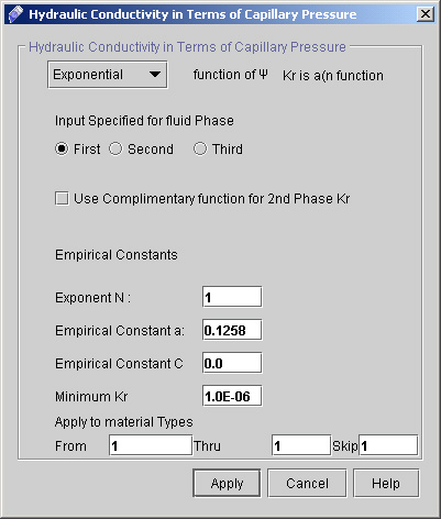
Fig - 3.2: Dialog window for Hydraulic conductivity.

5. Click "Apply".
6. Close the Multiphase characteristics dialog window by clicking "Close" button.

32) Now Close the Advanced solid Matrix Properties dialog window by clicking "Close" button on it.

33) Click "Next >>" to reach the Source & Sink Specification dialog window. (see fig 3.3)

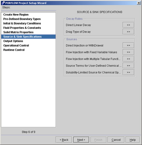
Fig - 3.3: Source & Sink Specification dialog.

34) Go to "Direct Injection or WithDrawal >>". A dialog window appears. Specify the values as:

1. Select dependent variable as P.
2. Check Source Strength per element and Strength as Specified.
3. Specify Region as SOURCE.
4. Select Value as Constant and enter 0.000525 in the text field. (See fig 3.4).



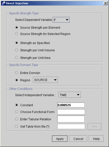
Fig - 3.4: Direct Injection dialog window

5. Click "Apply".

35) Click "Next >>" to go to Output Options dialog window (see fig 3.5)

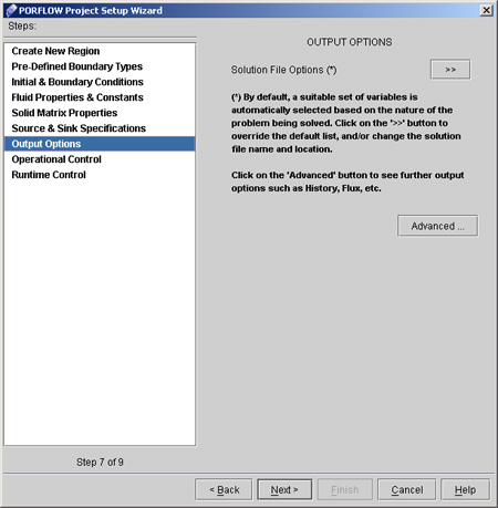
Fig - 3.5: Output Options dialog window

36) Go to "Solution File Options >>". A dialog window appears. In this dialog choose the values as:

1. Select Solution Options as "Customize Solution File Options".
2. Select "Formatted (ASCII)" and Enter the file name with extension .sav (default name is already there).
3. Select the variables as p.
4. Select print frequency as At the end only as shown in Fig 3.6.



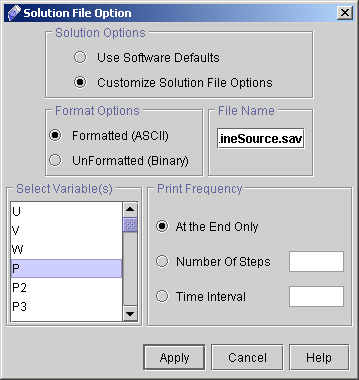
Fig - 3.6: Solution File option

5. Click "Apply".

37) Now go to Advanced option in Output options dialog window. You will find the following Dialog (fig 3.7)

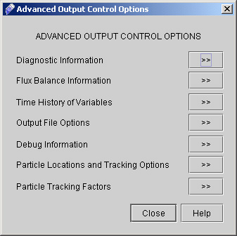
Fig - 3.7: Advanced Output Control Options

38) Click "Diagnostic Information >>" option to specify the diagnostic node at (20,62) and frequency of diagnostic information as 100.

39) Enter the value as shown in fig 3.8 and click "Apply".

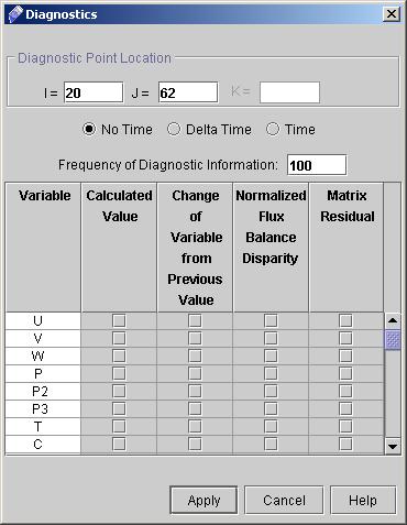
Fig - 3.8: Diagnostic dialog

1 2 3 4 5 6

# Back to CFDStudio/PORFLOW Tutorials Page

Related Links:

# PORFLOW Applications
# PORFLOW Express
# PORFLOW Publications
# PORFLOW Users
# PORFLOW Price List
# Request CFDStudio/PORFLOW Demo
# CFDStudio/PORFLOW Tutorials
# PORFLOW Manual
# PORFLOW Validation Report