1 2 3 4 5 6

11) Although you can come back to this panel to specify regions at a later stage, it is generally good practice to create any regions that will be used throughout the wizard - i.e., for specifying boundary / initial conditions or field variables, as well as sources - at this stage. We will specify most of the boundary conditions at the entire boundary domain, so we need not create any regions for that purpose. We will create two regions however, one for the SOURCE command, and the other to have output in particular domain.

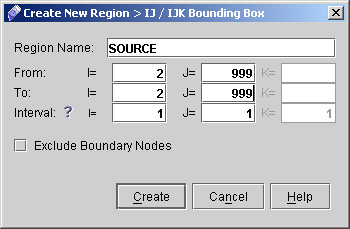
12) First we will create a point to represent the source. Click "IJ/IJK Bounding Box >>". A dialog window appears as shown in fig 1.8

Fig - 1.8: IJ/IJK Bounding Box

1. Enter the Region Name as SOURCE.
2. Enter the value of IJ (2,999) to IJ (2,999)
3. Click "Create".

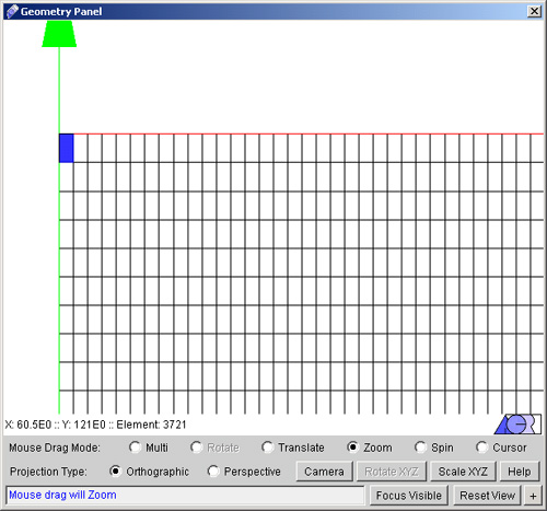
The created region after zooming it is shown on fig 1.9

Note: When we enter 999 as the value of I/J it means that it will take highest number (62 for present case) of indices in that direction otherwise instead of this we can specify maximum number of indices in respective direction that is 62 in J direction for the present case.

Fig - 1.9: Created Source

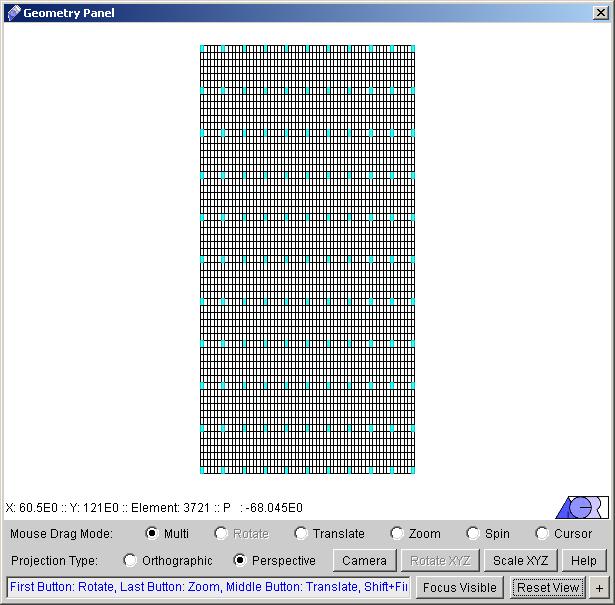
13) The second region will be generated to specify as the problem output region. Click again "IJ/IJK Bounding Box".

1. Enter the Region Name as OUTREG in text field.
2. Enter the value from IJ (1,1) to IJ (999,999)
3. Specify the interval 6 for I and 6 for J.
4. Click "Create".

the created region is shown in fig 2.0

Fig - 2.0: Created Region

We now have 2 regions that we can use during our problem setup. Note that you can select which one of these regions to view using the combo box on the top right of the main window

14) Click "Next >" in the wizard dialog to reach the "Pre-defined Boundary types". Here one can define boundary types like inlets, outlets, walls, periodic or symmetry boundaries .The problem we are setting does not have any explicit boundary types to set so we will not work on any of these options. Note that by default all domain boundaries are treated as open boundaries, so we will go with the defaults.

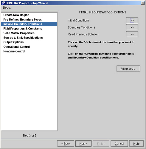
15) Click "Next >" to reach "Initial & Boundary Conditions" (See fig 2.1). We will provide starting values for the problem by setting initial pressure p as a linear function of y.

Fig - 2.1: Window for Initial & Boundary Conditions

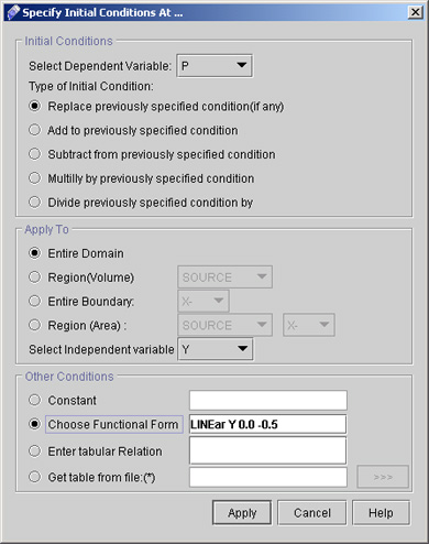
16) Click "Initial Conditions >>". A dialog box appear as shown in fig 2.3. Set the initial condition for P as follows

1. Select Dependent Variable as P.
2. Check Replace previously specified condition (if any).
3. Apply to "Entire Domain".
4. Select Independent Variable as Y.
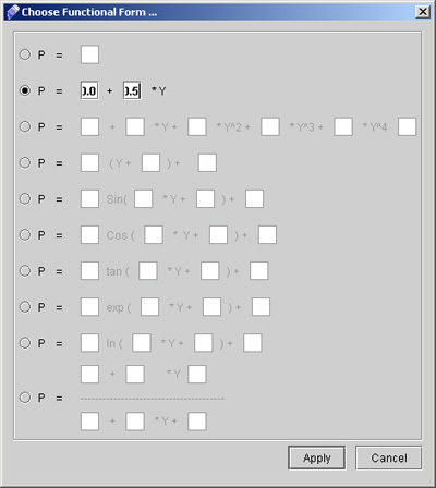
5. Check Choose Functional Form. A dialog window appears to specify the initial condition as a function of Y. Check the second box and enter the values as 0.0 and -0.5 in corresponding box and click "Apply" (see the fig 2.2).



Fig - 2.2: Dialog window to specify the functional form

6. The filled Initial conditions dialog window will be as shown in Fig 2.3



Fig 2.3 Initial Conditions dialog window

7. Click "Apply".

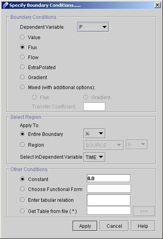
17) Now Click "Boundary Conditions >>" option in order to set the top, the left and the right boundary as no flow boundaries.

1. Select the dependent Variable as P.
2. Check Flux as type of boundary condition.
3. Apply to Entire Boundary at X-.
4. Leave the Time as independent variable as we are going to specify constant value of flux so there will be no effect of this parameter.
5. Select Constant and enter the value 0.0 in the text filed. (see Fig 2.4).



Fig - 2.4: Boundary Conditions dialog window

6. Click "Apply".

1 2 3 4 5 6

 

# Back to CFDStudio/PORFLOW Tutorials Page

 

Related Links:

# PORFLOW Applications
# PORFLOW Express
# PORFLOW Publications
# PORFLOW Users
# PORFLOW Price List
# Request CFDStudio/PORFLOW Demo
# CFDStudio/PORFLOW Tutorials
# PORFLOW Manual
# PORFLOW Validation Report