|


|
ACRi -- Analytic & Computational Research, Inc.
|
ACRi Unstructured Data Formats General Notes:
For a list of 3rd party grid generators that are compatible with ACRi software, please see the respective entry in the Frequently Asked Questions section. This document describes the file formats for using version 5.5 of the ACRi CFD solvers with unstructured meshes. However, future versions of ACRi software will be compatible with the data formats described here. Additionally, the specifications for regions, boundaries, and periodic pairs remain same in the next version of the solvers. This description consists of the actual data formats as well as the input commands that are needed to work with version 5.5 unstructured meshes. Highlights:
The unstructured data is specified via a mandatory commands file, a mandatory vertex (coordinates) file, a mandatory connectivity (element) file and an optional auxiliary connections (local refinement, or split connectivity) file. The formats are described below. MODE 1: Vertex Connectivity for Quad or Hex Elements The element to vertex connectivity is specified. The file must contain as many records as the number of elements specified on the GRID command. Each record consists of the element number followed by 4 (for 2D) or 8 (for 3D) vertex numbers of the element corners. Each record is read by the FORTRAN statement: For 2D geometry, the vertices must be specified in a counter-clock wise fashion in the x-y plane, such that the local (x, h) and the direction normal to the plane form a right handed system. For 3D geometry, the vertices on "bottom" side must be specified first (in counter-clockwise order) followed by the corresponding vertices on "top" side, such that the local (x, h, z) direction forms a right handed system. (Any side may be chosen as the "bottom", then the topologically opposite side is considered to be the "top"). The local (x, h, z) direction for each element is defined by the order in which the vertices appear on this record. The local x axis is oriented from vertex 1 to vertex 2, the h axis from vertex 1 to vertex 4, and the z axis from vertex 1 to vertex 5. These then determine the local side number (1, 2, 3, 4) or the local X-, X+, Y-, Y+, Z-, Z+ sides which are used to specify the boundary and boundary conditions. These concepts are illustrated in Figures 1 and 2. This is the default option. COMMENTS: An unstructured mesh is defined by: EXAMPLES: CONNectivity information on file "VERT2ELM.CNC"
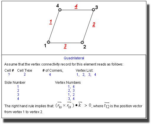
Figure 1: Relation between Vertex Numbers and Side Numbers for a Quadrilateral illustrating the application of the right hand rule. (2D only).
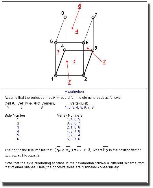
Figure 2: Relation between Vertex Numbers and Side Numbers for a Hexahedron illustrating the application of the right hand rule. (3D only). MODE 2: Vertex Connectivity for Mixed Hybrid Elements. The element to vertex connectivity is specified for a grid with mixed type of elements. Currently 6 different types of elements are allowed. These are given in the Table below.
The file must contain as many records as the number of elements specified on the GRID command. Each record must specify (in order), the element number, element type (given in the Table above), the total number of vertices for that element (given in Table above) and the vertex numbers for the element corners. Each record is read by the FORTRAN statement: Schematic of each element type and its connectivity describing the relationship of the local side numbering to the vertex connectivity is illustrated in Figures 1 through 6. EXAMPLES: CONNectivity for HYBRID elements on file "MIXED_ELEMENTS.CNC"
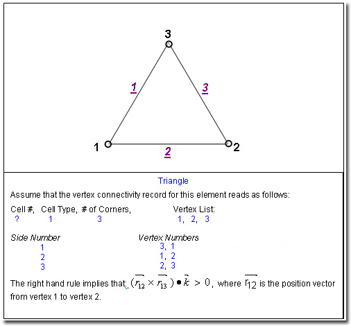
Figure 3: Relation between Vertex Numbers and Side Numbers for a Triangle illustrating the application of the right hand rule. (2D only).
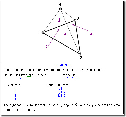
Figure 4: Relation between Vertex Numbers and Side Numbers for a Tetrahedron illustrating the application of the right hand rule. (3D only).
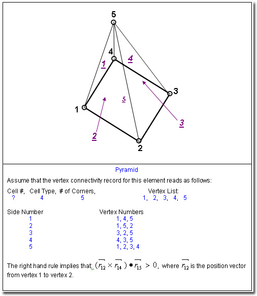
Figure 5: Relation between Vertex Numbers and Side Numbers for a Pyramid illustrating the application of the right hand rule. (3D only).
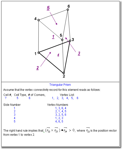
Figure 6: Relation between Vertex Numbers and Side Numbers for a Triangular Prism illustrating the application of the right hand rule. (3D only). MODE 3: Connectivity for Quad or Hex Elements with Split Sides The vertex and element connectivity for the split elements is specified. This is a supplementary mode of the command to enable local grid refinement or adaptation of the mesh in selected parts of the domain, based on solution features. (Split sides are element sides with more than one attached neighboring element). It can be used in conjunction with Mode 1 but is not available with Mode 2 of the command. By default all ACRi Software Tools assume that each element is connected to 4 other elements in 2D and 6 other element in 3D geometry. However if the grid is locally refined then a element may be split into multiple "child" elements and some of the elements may be connected to more than the default number of neighboring elements. This supplementary connectivity is specified in the following manner. The 1st record in the file consists of a header with two numbers: the number of split elements and the total number of data items in the rest of the file. The header is followed by a number of sets of data equal to the number of split elements. The 1st record of each set consists of the element number that is split followed by a side index for each side (4 for 2D and 6 for 3D) of the element which denotes the number of neighboring elements (if > 1) connected to that face. The index is zero if there is only one element connected to the side (no split). This record is followed by a list of element numbers that adjoin the split side in the order of the side index. The final record of the set consists of the local side number (from 1 to 6) for the adjoining elements that are attached to the split side. The entire file is read in using the following two FORTRAN statements: EXAMPLE:
If the ( Mode 1 ) vertex connectivity for the above mesh is as follows:
Then the SPLIt connectivity command is: CONNectivity SPLIT on file "SPLIT.CON." Contents of the file SPLIT. CON are: (the text on the right is for clarity and must NOT be present in the file)
Region Selection (Version 4.00 and above) A region can be selected by grouping a LIST of elements and giving them a unique name. In example 2, the elements 14, 18, 20, 22, 24 have been grouped into a list and given a name SAMPLE1 as follows:
Boundary Selection (Version 4.00 and above) Boundary surfaces can be selected by grouping them into a PAIRed list and giving them a unique name. In example 2, the right boundary is defined by:
Periodic Pairs (Version 4.00 and above) Periodic boundaries are defined by providing pairs of matching boundary faces in a file (typical extension .per). Each line of the file contains four integers Element No. Face No. Matching Element No. Matching Face No. See Example 2. Radial Coordinate System In a cylindrical system, some restrictions on the element orientations apply such that faces 3 and 4 are perpendicular to the global R direction and, in 3D, faces 5 and 6 are perpendicular to the global THETA direction. A vector from the centroid of face 3 to the centroid of face 4 should be approximately aligned with the unit vector in the R direction at the element centroid. Command Input Command input is accomplished via the FREEFORM™ language. For CFDStudio™ users, these commands are generated automatically. Commands start on column 1 of a line and consist of a keyword, modifiers, numeric, separator, terminator, and comment fields. The typical file extensions for the commands file are ".inp", or ".q1" (all lower case). An unstructured mesh is processed using the GRID, CONNectivity, and COORdinate commands. The syntax for the GRID command consists of the keyword GRID with modifiers UNST, THRE (for 3D only), and a numeric field denoting the number of elements. Thus for a 2D problem with 30,000 elements, the command is: Note that only the first four characters in a keyword or modifier are significant. The rest of the input is usually retained to make use of the self documenting feature of the FREEFORM™ language. The syntax for the CONNectivity command is: The syntax for the COORdinate command is: Regions are defined by grouping elements with the LOCAte LIST command as follows, Boundaries are defined by grouping boundary faces with the LOCAte PAIR command as follows, The appropriate face numbers are listed in Table 1(a) for 2D and Table 1(b) for 3D. Example 1 Figure 2 below shows a typical unstructured mesh to be used for this example.
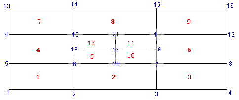
Figure 8: Ordering of the unknowns (element numbers in boxes), vertex numbers and face numbers. The arrangement of the elements forms an 'O' grid. Elements 1,3,5 and 9 have split faces formed due to local refinement. The arrows indicate the local '4' orientation of each element. Vertex File, Example-1.xyz:
Connectivity File, Example-1.cnc:
Commands in File "Example-1.inp":
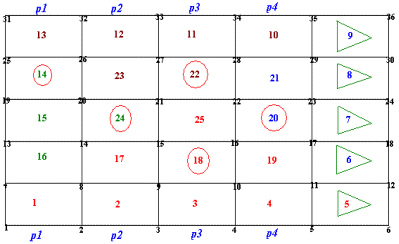
Example 2 Figure. 9 below shows another unstructured mesh to be used for Example 2.
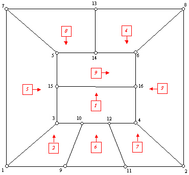
Figure 9. An example mesh to illustrate setting up boundary definitions. The faces labeled p1 .. p4 form periodic pairs. The circled elements are gathered into a sub-region using the "LOCAte LIST" command. The right boundary, composed of the elements with the arrow heads pointing to the boundary, is defined using a "LOCAte PAIR" command.
Commands in File "Example-2.inp": GRID UNSTructured 25 elements CONNectivity 'Example-2.cnc' COORdinate VERTices X Y 'Example-2.xyz' PERIodic 'Example-2.per' LOCAte LIST ID=SAMPLE114, 18, 20, 22, 24LOCAte PAIR ID=RIGHTBC5, 2 ; 6, 3 ; 7, 3 ; 8, 3 ; 9, 3 ; | |||||||||||||||||||||||||||||||||||||||||||||||||||||||||||||||||||||||||||||||||||||||||||||||||||||||||||||||||||||||||||||||||||||||||||||||||||||||||||||||||||||||||||||||||||||||||||||||||||||||||||||||||||||||||||||||||||||||||||||||||||||||||||||||||||||||||||||||||||||||||||||||||||||||||||||||||||||||||||||||||||||||||||||||||||||||||||||||||||||||||||||||||||||||||||||||||||||||||||||||||||||||||||||||||||||||||||||||||||||||||||||||||||||||||||||||||||||||||||||||||||||||||||||||||||||||||||||||||||||||||||||||||||||||||||||||||||||||||||||||||||||||||||||||||||||||||||||||||||||||||||||||||||||||||||||||||||||||||||||